Beyond Averages: How Monte Carlo simulation reveals the true risks in a system

The Danger of Averages

One of the core and intractable challenges when simulating an uncertain future is the problem of quantisation: when an all-or-nothing outcome is distilled into an average that distorts the true meaning of the data.

Though it’s often easier to say “Investing in this asset has an average return of 110%”, most systems do not converge neatly on an average value. Further, when the personal or financial cost of “getting unlucky” is disproportionately greater than any size of profit, looking just at averages no longer suffices.

Investing your life’s savings in a promising new market may net you a 150% return on average, but that might only be because the small chance of returning >500% outweighs the small but tangible chance of returning 0%.

When more wealth means a greater ability to accrue more wealth (see the Pareto Principle), losing almost everything on a bad investment can spell disaster, and no simple estimation of average returns will account for this.

Using Simulations

This is why Monte Carlo simulation is essential for modelling such systems, where quantised, all-or-nothing events stack up to produce diverse outcomes.

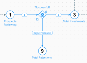
Capital investment is a prime example:

 

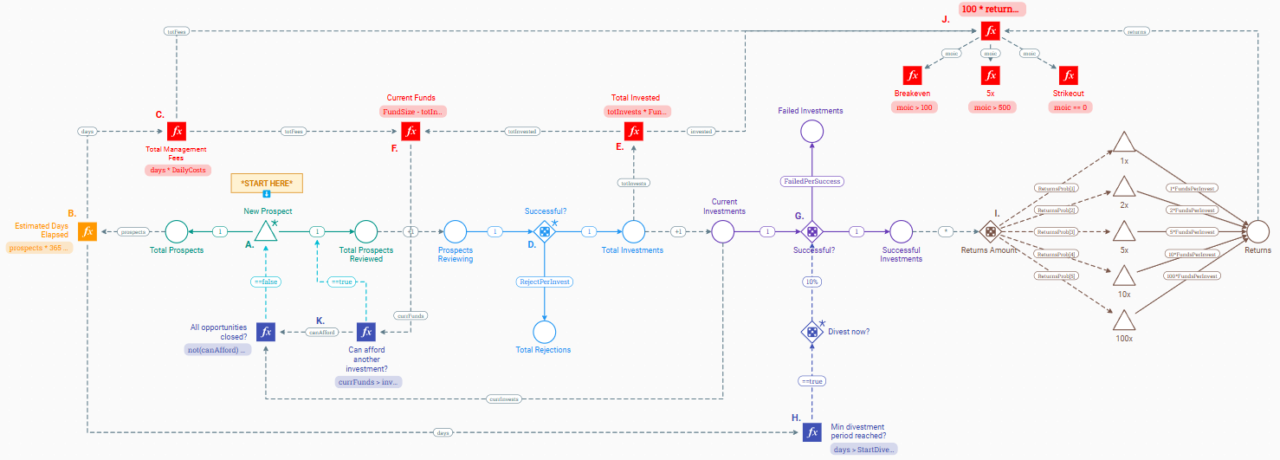
In the model above, we simulate a venture capital fund, in which an investment firm sets aside a certain amount of funds to invest in prospective businesses. Each business, or prospect, may be given funding or rejected, and their return on investment may take a range of values: 1x the original investment, 2x, 5x, 10x, 100x; or, crucially, 0x (i.e. failing to return anything).

Our key output of interest is the Multiple on Invested Capital (MOIC), which estimates the total return on investment for all prospects in the fund. This measure accounts not only for the actual amount invested in each prospect, but also any management costs associated with running the fund, such as investor salaries. This means that the investment firm can still net a loss if they find no worthy investments.

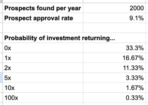
In whatever model or average calculation we use, we make several crucial assumptions, such as the average approval rate of prospects seeking funding, or the odds of an investment returning 0x, 1x, 2x, etc. These assumptions are effectively claims about the future, albeit an “average, most likely future”. But even if a certain outcome is the most likely of all other outcomes, it does not mean that the odds for that outcome are strong. Ultimately, the best assumption is merely the one that’s least likely to be wrong.

Versus Averages

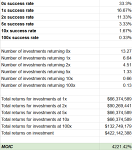
If, having made these assumptions, we were to simply multiply all these averages together, we would find an extremely positive picture. In the example above, this is because, despite a 100x return on investment being a quantised, all-or-nothing event, we’ve treated it as a pure mathematical average.

Thus, if the fund has, on average, 0.13 investments return 100x, we still end up returning 13x. That gets us a MOIC of over 4000%.

Since we can’t have 0.13 of an investment, we need to move beyond averages and look at what happens when an event does, or does not happen.

The benefit of Monte Carlo simulation is that we can keep using high-level averages as a starting point, and yet still obtain representative data with them.

The Model

In the model, when we simulate a success rate, such as the rate at which prospects are funded or rejected, we use randomness to generate a quantised, yes/no outcome. Each time a new prospect is reviewed, we roll a weighted dice to determine whether they are accepted or rejected (where the odds of success or failure are equal to our assumed values). This means that each time we run the model from scratch, each prospect may turn out differently.

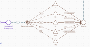
This practice is especially relevant for rare events with disproportionate outcomes, like our 100x return on investment event. In the model, each investment has a 0.33% chance of returning 100x (or 1%, after separating out the chance of 0x). This means that in most cases, there are zero investments that return 100x. Consequently, MOIC is rarely so high as in our average estimation.

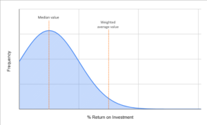
On running Monte Carlo simulations (i.e. Predictions) with the Machinations model, we find a spread of results:

Though the average MOIC is still over 100% (i.e. a positive return on investment), even this simple average is deceptive: this average is not the most likely outcome. It is in fact just an abstract statistical value that holds little practical value.

The true, most likely outcome is better represented by the histogram, or even just the median. In this case, the most likely outcome is a MOIC of less than 100% – in other words, a net loss. This stands in stark contrast to both our original estimation, and the model’s own mean value.

Conclusion

Observing the spread of results, the model has shown that the fund is disproportionately more likely to lose money. Since less money for an investment firm means less investment opportunities in the future, the risk analysis must address the full distribution and not just the average.

More generally, the venture capital model has revealed how using a simple weighted average to infer the most likely outcome would not only give the wrong result, but might also lead to a totally different decision being made. Using the Monte Carlo method, we can better understand the full breadth of outcomes and, by extention, better understand the all-round best decision to make.