Urban Mobility: Transportation and Infrastructure Planning Perfected

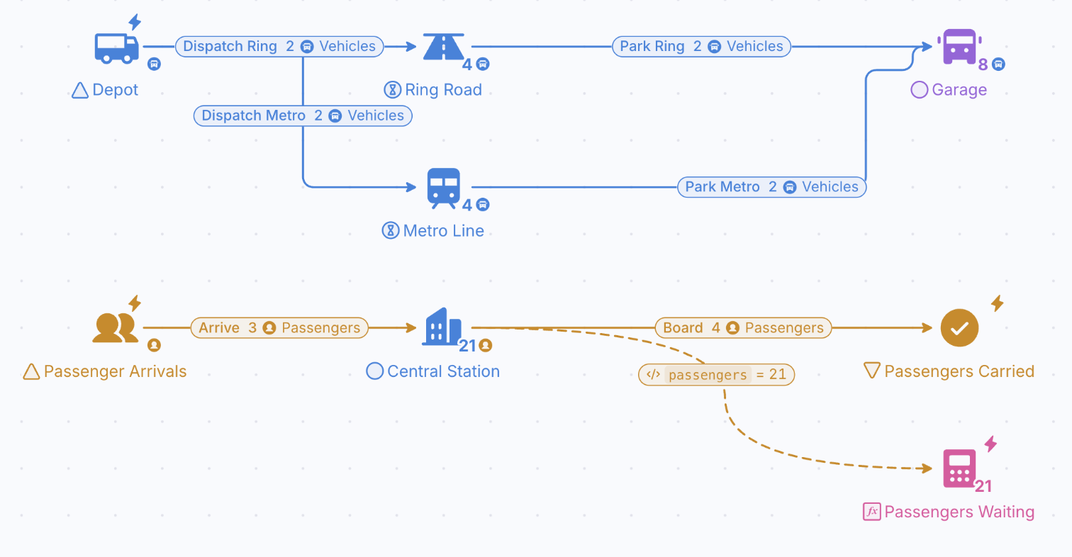
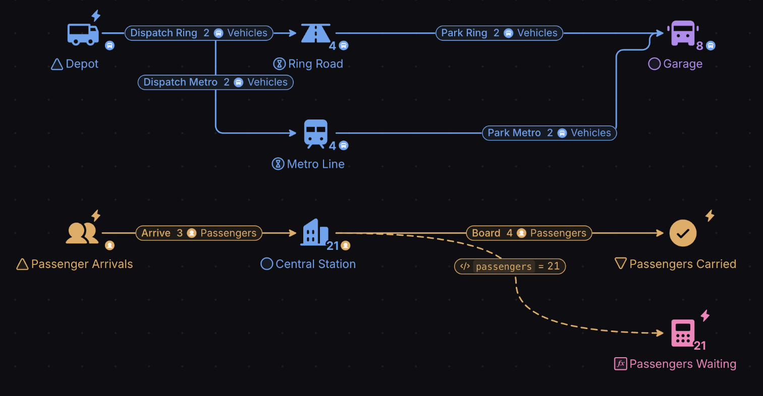
Transform your transport systems with advanced modeling and analysis for efficient and sustainable infrastructure.

Sign-up for free

Dedicated to Excellence and Compliance

Traffic Flow Simulation

Model the dynamics of vehicle movement through a network of roads, including intersections and traffic signals. Optimize traffic light timings and road layouts to reduce congestion and improve traffic flow.

Infrastructure Project Impact Analysis

Assess the potential impacts of new infrastructure projects, such as highways or bridges, on existing transportation networks. Predict changes in traffic patterns and identify potential bottlenecks or improvements in connectivity.

Public Transit System Design

Simulate the operation of buses, trains, and other public transit vehicles within a city. Plan routes, schedules, and frequencies to maximize coverage and minimize wait times for passengers.

Freight and Logistics Optimization

Model the transportation of goods through various modes, including trucks, trains, and ships. Optimize routes, schedules, and load management to improve the efficiency and reduce the cost of freight operations.

Shared Mobility Services

Simulate the operation and demand for shared mobility services such as ride-hailing, car-sharing, and bike-sharing, as well as the usage patterns of parking facilities. Plan service areas, optimize vehicle distribution, and improve service reliability.

Environmental Impact Assessment

Model the environmental impacts of transportation systems, including emissions and noise pollution. Evaluate the effectiveness of various mitigation strategies, such as green infrastructure or emission reduction technologies.

Explore the largest

systems thinking community

in the World

34.1k Public Diagrams

54.8k Designers Profiles

CCO 1.0 Universal Public Domain Dedication Creative Commons license

Ready to Optimize?

Advance Urban Mobility with Machinations. Model, analyze, and improve your transportation systems for better traffic flow, safety, and environmental impact. Join industry leaders and set new standards in transportation excellence.

Get Started